The 5 Feature Selection Algorithms every Data Scientist should know

Data Science is the study of algorithms.
I grapple through with many algorithms on a day to day basis, so I thought of listing some of the most common and most used algorithms one will end up using in this new DS Algorithm series.
How many times it has happened when you create a lot of features and then you need to come up with ways to reduce the number of features.
We sometimes end up using correlation or tree-based methods to find out the important features.
Can we add some structure to it?
This post is about some of the most common feature selection techniques one can use while working with data.
Why Feature Selection?
Before we proceed, we need to answer this question. Why don’t we give all the features to the ML algorithm and let it decide which feature is important?
So there are three reasons why we don’t:
1. Curse of dimensionality — Overfitting

If we have more columns in the data than the number of rows, we will be able to fit our training data perfectly, but that won’t generalize to the new samples. And thus we learn absolutely nothing.
2. Occam’s Razor:
We want our models to be simple and explainable. We lose explainability when we have a lot of features.
3. Garbage In Garbage out:
Most of the times, we will have many non-informative features. For Example, Name or ID variables. Poor-quality input will produce Poor-Quality output.
Also, a large number of features make a model bulky, time-taking, and harder to implement in production.
So What do we do?

We select only useful features.
Fortunately, Scikit-learn has made it pretty much easy for us to make the feature selection. There are a lot of ways in which we can think of feature selection, but most feature selection methods can be divided into three major buckets
- Filter based: We specify some metric and based on that filter features. An example of such a metric could be correlation/chi-square.
- Wrapper-based: Wrapper methods consider the selection of a set of features as a search problem. Example: Recursive Feature Elimination
- Embedded: Embedded methods use algorithms that have built-in feature selection methods. For instance, Lasso and RF have their own feature selection methods.
So enough of theory let us start with our five feature selection methods.
We will try to do this using a dataset to understand it better.
I am going to be using a football player dataset to find out what makes a good player great?
Don’t worry if you don’t understand football terminologies. I will try to keep it at a minimum.
Here is the Kaggle Kernel with the code to try out yourself.
Some Simple Data Preprocessing
We have done some basic preprocessing such as removing Nulls and one hot encoding. And converting the problem to a classification problem using:
y = traindf['Overall']>=87
Here we use High Overall as a proxy for a great player.
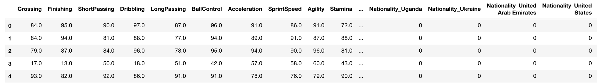
Our dataset(X) looks like below and has 223 columns.
1. Pearson Correlation
This is a filter-based method.
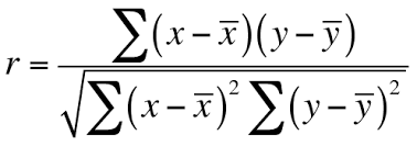
We check the absolute value of the Pearson’s correlation between the target and numerical features in our dataset. We keep the top n features based on this criterion.
def cor_selector(X, y,num_feats):
    cor_list = []
    feature_name = X.columns.tolist()
    # calculate the correlation with y for each feature
    for i in X.columns.tolist():
        cor = np.corrcoef(X[i], y)[0, 1]
        cor_list.append(cor)
    # replace NaN with 0
    cor_list = [0 if np.isnan(i) else i for i in cor_list]
    # feature name
    cor_feature = X.iloc[:,np.argsort(np.abs(cor_list))[-num_feats:]].columns.tolist()
    # feature selection? 0 for not select, 1 for select
    cor_support = [True if i in cor_feature else False for i in feature_name]
    return cor_support, cor_feature
cor_support, cor_feature = cor_selector(X, y,num_feats)
print(str(len(cor_feature)), 'selected features')
2. Chi-Squared
This is another filter-based method.
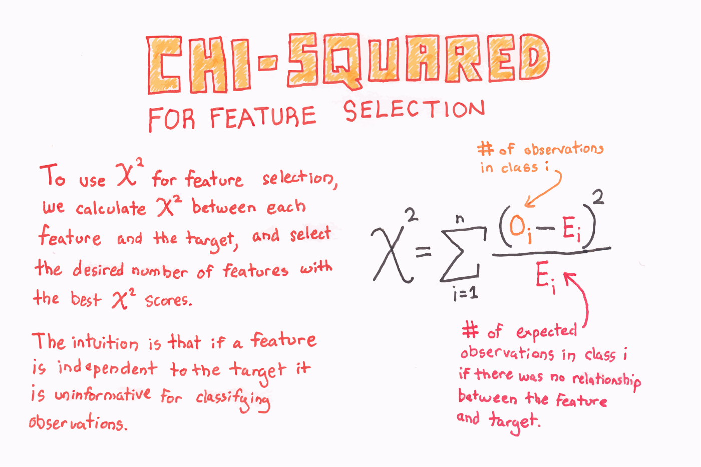
In this method, we calculate the chi-square metric between the target and the numerical variable and only select the variable with the maximum chi-squared values.
Let us create a small example of how we calculate the chi-squared statistic for a sample.
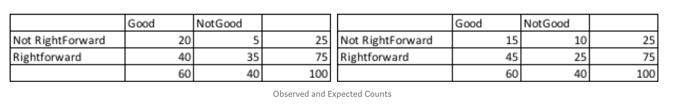
So let’s say we have 75 Right-Forwards in our dataset and 25 Non-Right-Forwards. We observe that 40 of the Right-Forwards are good, and 35 are not good. Does this signify that the player being right forward affects the overall performance?
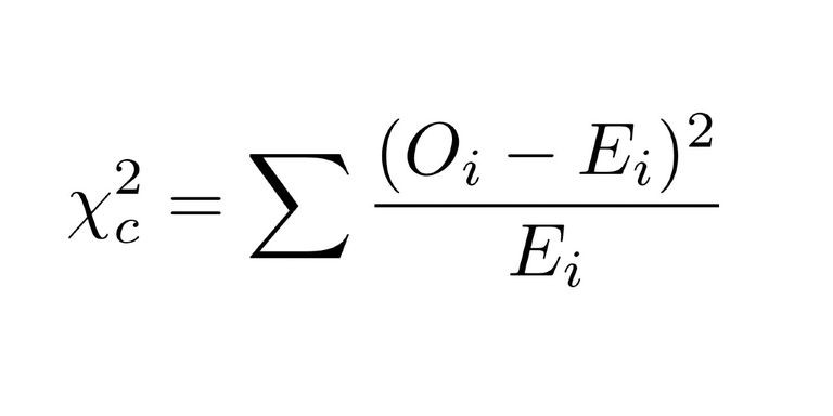
We calculate the chi-squared value:
To do this, we first find out the values we would expect to be falling in each bucket if there was indeed independence between the two categorical variables.
This is simple. We multiply the row sum and the column sum for each cell and divide it by total observations.
so Good and NotRightforward Bucket Expected value= 25(Row Sum)*60(Column Sum)/100(Total Observations)
Why is this expected? Since there are 25% notRightforwards in the data, we would expect 25% of the 60 good players we observed in that cell. Thus 15 players.
Then we could just use the below formula to sum over all the 4 cells:
I won’t show it here, but the chi-squared statistic also works in a hand-wavy way with non-negative numerical and categorical features.
We can get chi-squared features from our dataset as:
from sklearn.feature_selection import SelectKBest
from sklearn.feature_selection import chi2
from sklearn.preprocessing import MinMaxScaler
X_norm = MinMaxScaler().fit_transform(X)
chi_selector = SelectKBest(chi2, k=num_feats)
chi_selector.fit(X_norm, y)
chi_support = chi_selector.get_support()
chi_feature = X.loc[:,chi_support].columns.tolist()
print(str(len(chi_feature)), 'selected features')
3. Recursive Feature Elimination

This is a wrapper based method. As I said before, wrapper methods consider the selection of a set of features as a search problem.
From sklearn Documentation:
The goal of recursive feature elimination (RFE) is to select features by recursively considering smaller and smaller sets of features. First, the estimator is trained on the initial set of features and the importance of each feature is obtained either through acoef_attribute or through afeature_importances_attribute. Then, the least important features are pruned from current set of features. That procedure is recursively repeated on the pruned set until the desired number of features to select is eventually reached.
As you would have guessed, we could use any estimator with the method. In this case, we use
LogisticRegression, and the RFE observes the coef_ attribute of the LogisticRegression objectfrom sklearn.feature_selection import RFE
from sklearn.linear_model import LogisticRegression
rfe_selector = RFE(estimator=LogisticRegression(), n_features_to_select=num_feats, step=10, verbose=5)
rfe_selector.fit(X_norm, y)
rfe_support = rfe_selector.get_support()
rfe_feature = X.loc[:,rfe_support].columns.tolist()
print(str(len(rfe_feature)), 'selected features')4. Lasso: SelectFromModel
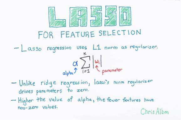
This is an Embedded method. As said before, Embedded methods use algorithms that have built-in feature selection methods.
For example, Lasso and RF have their own feature selection methods. Lasso Regularizer forces a lot of feature weights to be zero.
Here we use Lasso to select variables.
from sklearn.feature_selection import SelectFromModel
from sklearn.linear_model import LogisticRegression

embeded_lr_selector = SelectFromModel(LogisticRegression(penalty="l1"), max_features=num_feats)
embeded_lr_selector.fit(X_norm, y)

embeded_lr_support = embeded_lr_selector.get_support()
embeded_lr_feature = X.loc[:,embeded_lr_support].columns.tolist()
print(str(len(embeded_lr_feature)), 'selected features')
5. Tree-based: SelectFromModel

This is an Embedded method. As said before, Embedded methods use algorithms that have built-in feature selection methods.
We can also use RandomForest to select features based on feature importance.
We calculate feature importance using node impurities in each decision tree. In Random forest, the final feature importance is the average of all decision tree feature importance.
from sklearn.feature_selection import SelectFromModel
from sklearn.ensemble import RandomForestClassifier

embeded_rf_selector = SelectFromModel(RandomForestClassifier(n_estimators=100), max_features=num_feats)
embeded_rf_selector.fit(X, y)

embeded_rf_support = embeded_rf_selector.get_support()
embeded_rf_feature = X.loc[:,embeded_rf_support].columns.tolist()
print(str(len(embeded_rf_feature)), 'selected features')
We could also have used a LightGBM. Or an XGBoost object as long it has a
feature_importances_ attribute.from sklearn.feature_selection import SelectFromModel
from lightgbm import LGBMClassifier
lgbc=LGBMClassifier(n_estimators=500, learning_rate=0.05, num_leaves=32, colsample_bytree=0.2,
reg_alpha=3, reg_lambda=1, min_split_gain=0.01, min_child_weight=40)
embeded_lgb_selector = SelectFromModel(lgbc, max_features=num_feats)
embeded_lgb_selector.fit(X, y)
embeded_lgb_support = embeded_lgb_selector.get_support()
embeded_lgb_feature = X.loc[:,embeded_lgb_support].columns.tolist()
print(str(len(embeded_lgb_feature)), 'selected features')Bonus

Why use one, when we can have all?
The answer is sometimes it won’t be possible with a lot of data and time crunch.
But whenever possible, why not do this?
# put all selection together
feature_selection_df = pd.DataFrame({'Feature':feature_name, 'Pearson':cor_support, 'Chi-2':chi_support, 'RFE':rfe_support, 'Logistics':embeded_lr_support,
                                    'Random Forest':embeded_rf_support, 'LightGBM':embeded_lgb_support})
# count the selected times for each feature
feature_selection_df['Total'] = np.sum(feature_selection_df, axis=1)
# display the top 100
feature_selection_df = feature_selection_df.sort_values(['Total','Feature'] , ascending=False)
feature_selection_df.index = range(1, len(feature_selection_df)+1)
We check if we get a feature based on all the methods. In this case, as we can see Reactions and LongPassing are excellent attributes to have in a high rated player. And as expected Ballcontrol and Finishing occupy the top spot too.