Every time we are working with a dataset, our dataset represent a sample from a population. Using this sample, we can then try to understand it’s main patterns so that we can use it to make predictions on the whole population (even though we never had the opportunity to examine the whole population).
Let’s imagine we want to predict the price of a house given a certain set of features. We might be able to find online a dataset with all the house prices of San Francisco (our sample) and after performing some statistical analysis, we might be able to make quite accurate predictions of the house price in any other city in the USA (our population).
Datasets are composed of two main types of data: Numerical (eg. integers, floats), and Categorical (eg. names, laptops brands).
Numerical data can additionally be divided into other two categories: Discrete and Continue. Discrete data can take only certain values (eg. number of students in a school) while continuous data can take any real or fractional value (eg. the concepts of height and weights).
From discrete random variables, it is possible to calculate Probability Mass Functions, while from continuous random variables can be derived Probability Density Functions.
Probability Mass Functions gives the probability that a variable can be equal to a certain value, instead, the values of Probability Density Functions are not itself probabilities because they need first to be integrated over the given range.
There exist many different probability distributions in nature (Figure 1), in this article I will introduce you to the ones most commonly used in Data Science.
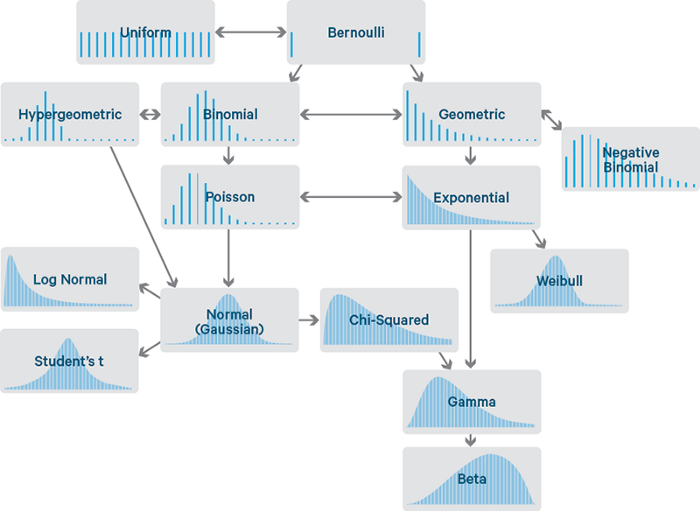
Figure 1: Probability Distributions Flowchart [1]
Throughout this article, I will provide code snippets on how to create each of the different distributions. If you are interested in additional resources, these are available in
this my GitHub repository.
First of all, let’s import all the necessary libraries:
| import pandas as pd |
| import numpy as np |
| import matplotlib.pyplot as plt |
| import scipy.stats as stats |
| import seaborn as sns |
Bernoulli Distribution
The Bernoulli distribution is one of the easiest distributions to understand and can be used as a starting point to derive more complex distributions.
This distribution has only two possible outcomes and a single trial.
A simple example can be a single toss of a biased/unbiased coin. In this example, the probability that the outcome might be heads can be considered equal to p and (1 - p) for tails (the probabilities of mutually exclusive events that encompass all possible outcomes needs to sum up to one).
In Figure 2, I provided an example of Bernoulli distribution in the case of a biased coin.
| probs = np.array([0.75, 0.25]) |
| face = [0, 1] |
| plt.bar(face, probs) |
| plt.title('Loaded coin Bernoulli Distribution', fontsize=12) |
| plt.ylabel('Probability', fontsize=12) |
| plt.xlabel('Loaded coin Outcome', fontsize=12) |
| axes = plt.gca() |
| axes.set_ylim([0,1]) |
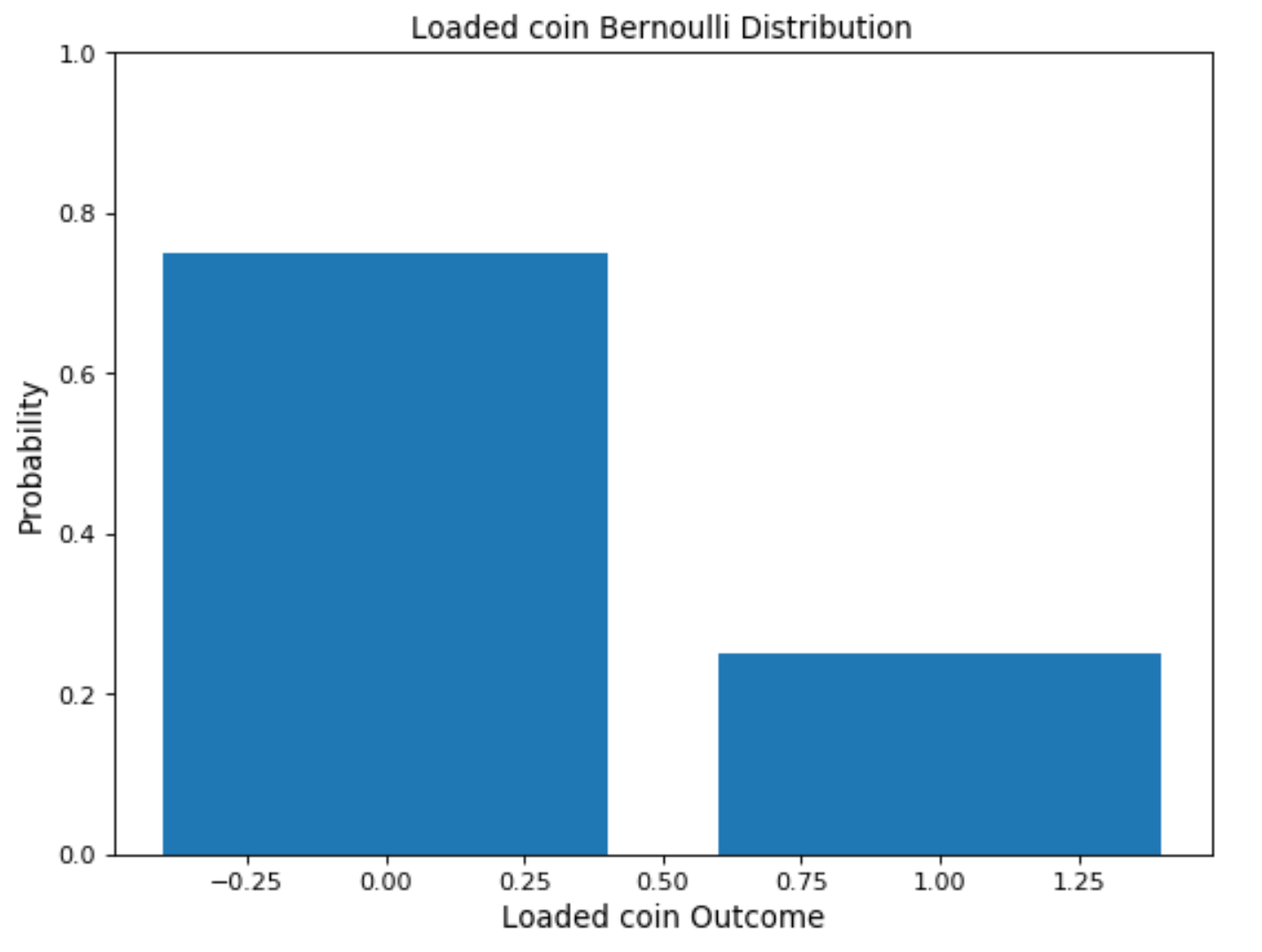
Figure 2: Bernoulli distribution biased coin
Uniform Distribution
The Uniform Distribution can be easily derived from the Bernoulli Distribution. In this case, a possibly unlimited number of outcomes are allowed and all the events hold the same probability to take place.
As an example, imagine the roll of a fair dice. In this case, there are multiple possible events with each of them having the same probability to happen.
| probs = np.full((6), 1/6) |
| face = [1,2,3,4,5,6] |
| plt.bar(face, probs) |
| plt.ylabel('Probability', fontsize=12) |
| plt.xlabel('Dice Roll Outcome', fontsize=12) |
| plt.title('Fair Dice Uniform Distribution', fontsize=12) |
| axes = plt.gca() |
| axes.set_ylim([0,1]) |
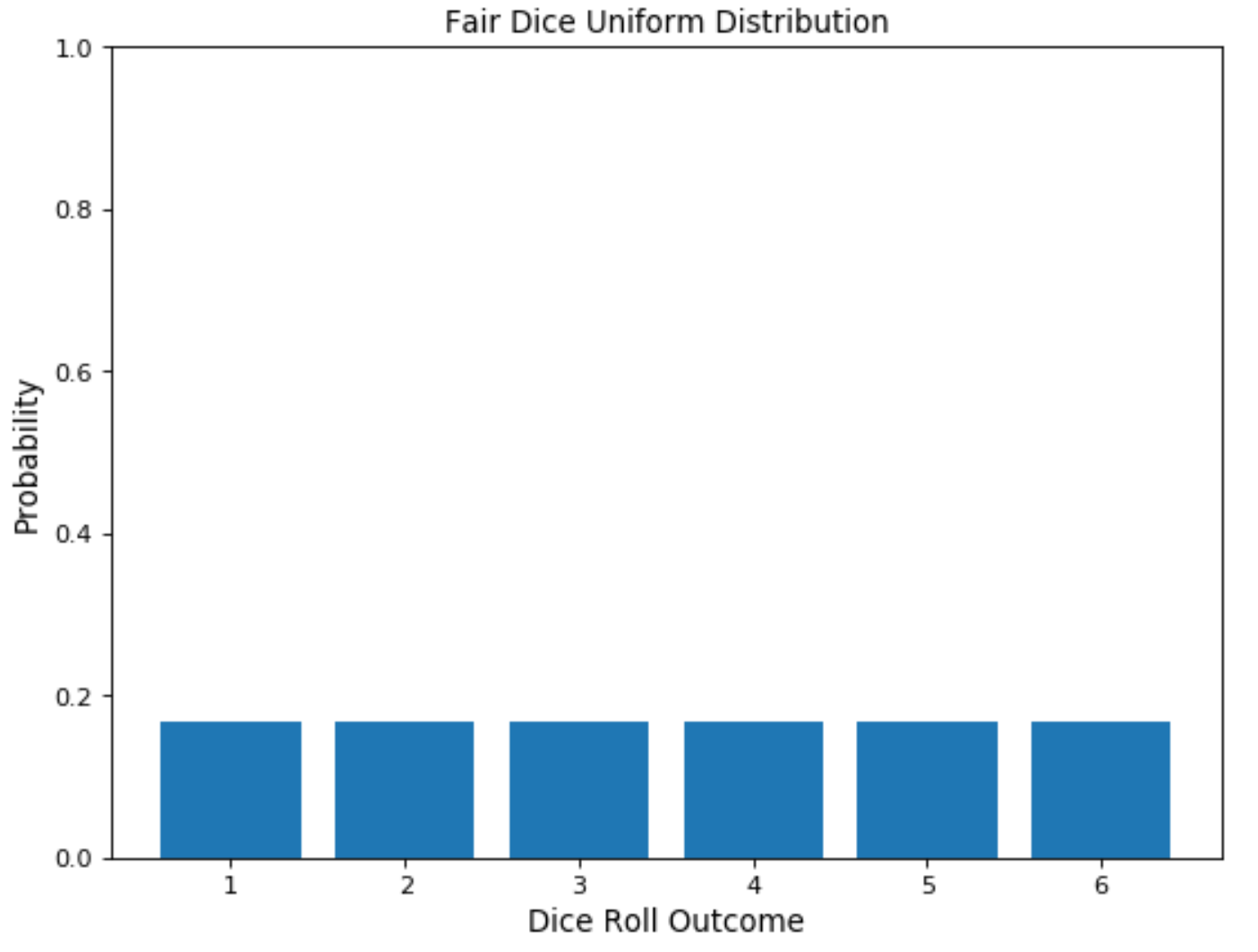
Figure 3: Fair Dice Roll Distribution
Binomial Distribution
The Binomial Distribution can instead be thought as the sum of outcomes of an event following a Bernoulli distribution. The Binomial Distribution is therefore used in binary outcome events and the probability of success and failure is the same in all the successive trials. This distribution takes two parameters as inputs: the number of times an event takes place and the probability assigned to one of the two classes.
A simple example of a Binomial Distribution in action can be the toss of a biased/unbiased coin repeated a certain amount of times.
Varying the amount of bias will change the way the distribution will look like (Figure 4).
| # pmf(random_variable, number_of_trials, probability) |
| for prob in range(3, 10, 3): |
| x = np.arange(0, 25) |
| binom = stats.binom.pmf(x, 20, 0.1*prob) |
| plt.plot(x, binom, '-o', label="p = {:f}".format(0.1*prob)) |
| plt.xlabel('Random Variable', fontsize=12) |
| plt.ylabel('Probability', fontsize=12) |
| plt.title("Binomial Distribution varying p") |
| plt.legend() |
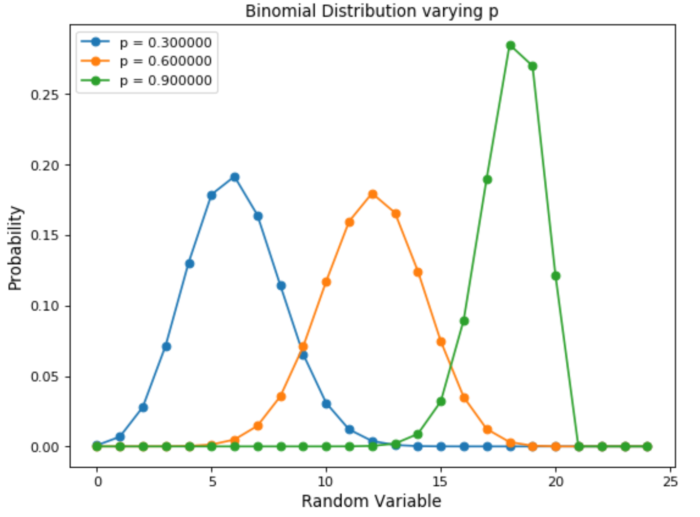
Figure 4: Binomial Distribution varying event occurrence probability
The main characteristics of a Binomial Distribution are:
- Given multiple trials, each of them is independent of each other (the outcome of one trial doesn’t affect another one).
- Each trial can lead to just two possible results (eg. winning or losing), which have probabilities p and (1 - p).
If we are given the probability of success (p) and the number of trials (n), we can then be able to calculate the probability of success (x) within these n trials using the formula below (Figure 5).
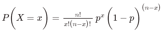
Figure 5: Binomial Distribution Formula [2]
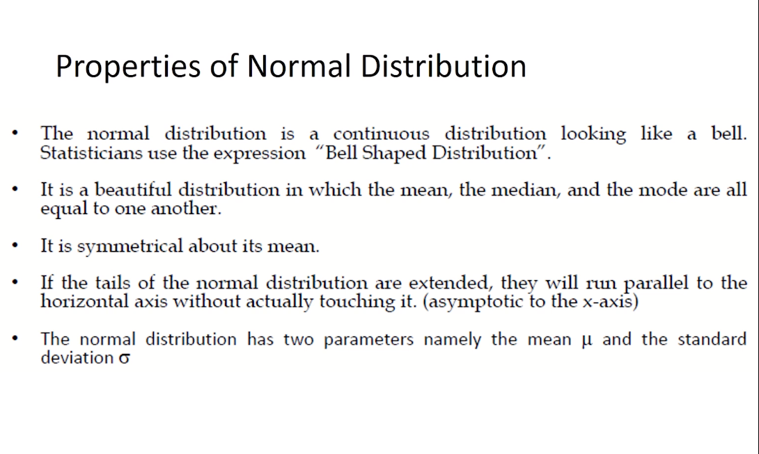
Normal (Gaussian) Distribution
The Normal Distribution is one of the most used distributions in Data Science. Many common phenomena that take place in our daily life follows Normal Distributions such as: the income distribution in the economy, students average reports, the average height in populations, etc… In addition to this, the sum of small random variables also turns out to usually follow a normal distribution (Central Limit Theorem).
“In probability theory, the central limit theorem (CLT) establishes that, in some situations, when independent random variables are added, their properly normalized sum tends toward a normal distribution even if the original variables themselves are not normally distributed.”
| n = np.arange(-50, 50) |
| mean = 0 |
| normal = stats.norm.pdf(n, mean, 10) |
| plt.plot(n, normal) |
| plt.xlabel('Distribution', fontsize=12) |
| plt.ylabel('Probability', fontsize=12) |
| plt.title("Normal Distribution") |
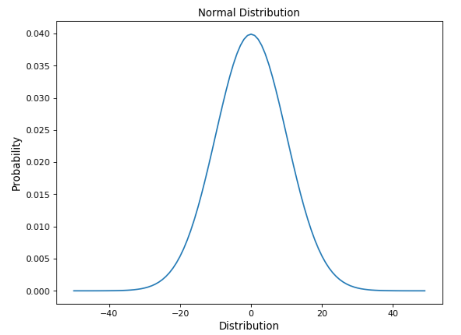
Figure 6: Gaussian Distribution
Some of the characteristics which can help us to recognise a normal distribution are:
- The curve is symmetric at the centre. Therefore mean, mode and median are all equal to the same value, making distribute all the values symmetrically around the mean.
- The area under the distribution curve is equal to 1 (all the probabilities must sum up to 1).
A normal distribution can be derived using the following formula (Figure 7).
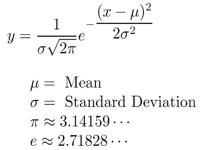
Figure 7: Normal Distribution Formula [3]
When using Normal Distributions, the distribution mean and standard deviation plays a really important role. If we know their values, we can then easily find out the probability of predicting exact values by just examining the probability distribution (Figure 8). In fact, thanks to the distribution properties, 68% of the data lies within one standard deviation of the mean, 95% within two standard deviations of the mean and 99.7% within three standard deviations of the mean.
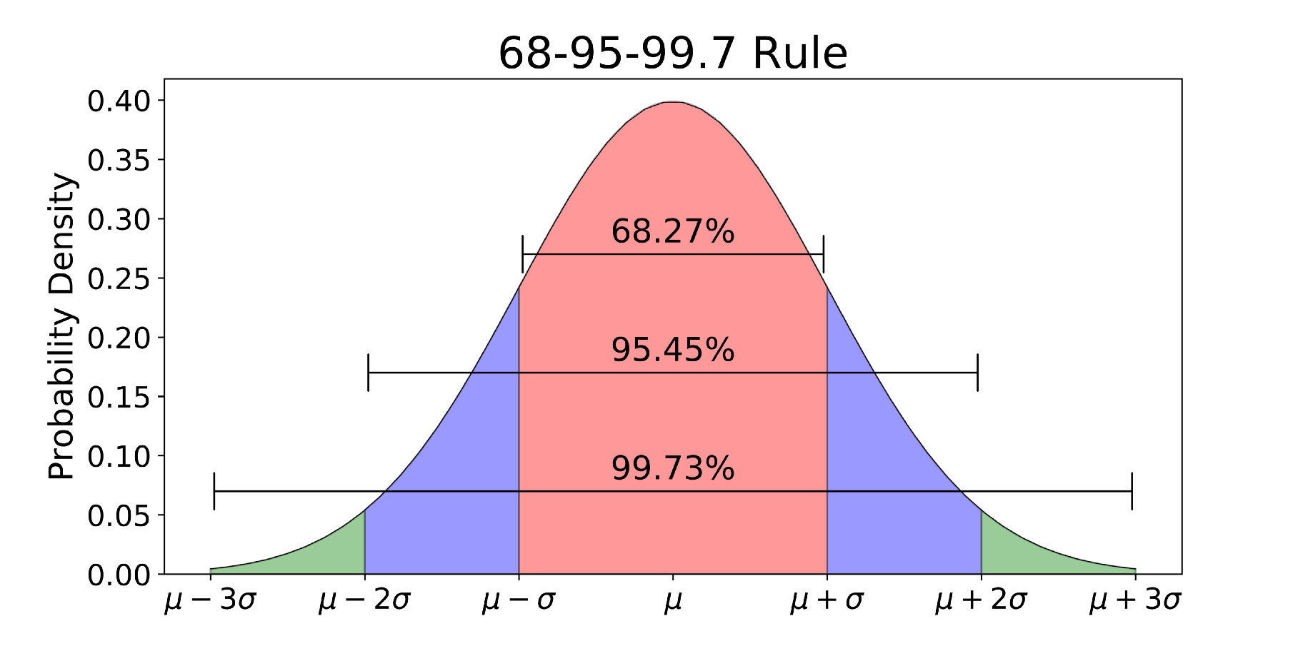
Figure 8: Normal Distribution 68–95–99.7 Rule [4]
Many Machine Learning models are designed to work best-using data that follow a Normal Distribution. Some examples are:
- Gaussian Naive Bayes Classifier
- Linear Discriminant Analysis
- Quadratic Discriminant Analysis
- Least Squares based regression models
Additionally, it is also possible in some cases to transform not-normal data into a normal form by applying transformations such as logarithms and square roots.
Poisson Distribution
Poisson Distributions are commonly used to find the probability that an event might happen or not knowing how often it usually occurs. Additionally, Poisson Distributions can also be used to predict how many times an event might occur in a given time period.
Poisson Distributions are for example frequently used by insurance companies to conduct risk analysis (eg. predict the number of car crash accidents within a predefined time span) to decide car insurance pricing.
When working with Poisson Distributions, we can be confident of the average time between the occurrence of different events, but the precise moment an event might take place is randomly spaced in time.
A Poisson Distribution can be modelled using the following formula (Figure 9), where λ represents the expected number of events which can take place in a period.
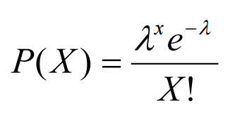
Figure 9: Poisson Distribution Formula [5]
The main characteristics which describe Poisson Processes are:
- The events are independent of each other (if an event happens, this does not alter the probability that another event can take place).
- An event can take place any number of times (within the defined time period).
- Two events can’t take place simultaneously.
- The average rate between events occurrence is constant.
In Figure 10, is shown how varying the expected number of events which can take place in a period (λ) can change a Poisson Distribution.
| # n = number of events, lambd = expected number of events |
| # which can take place in a period |
| for lambd in range(2, 8, 2): |
| n = np.arange(0, 10) |
| poisson = stats.poisson.pmf(n, lambd) |
| plt.plot(n, poisson, '-o', label="λ = {:f}".format(lambd)) |
| plt.xlabel('Number of Events', fontsize=12) |
| plt.ylabel('Probability', fontsize=12) |
| plt.title("Poisson Distribution varying λ") |
| plt.legend() |
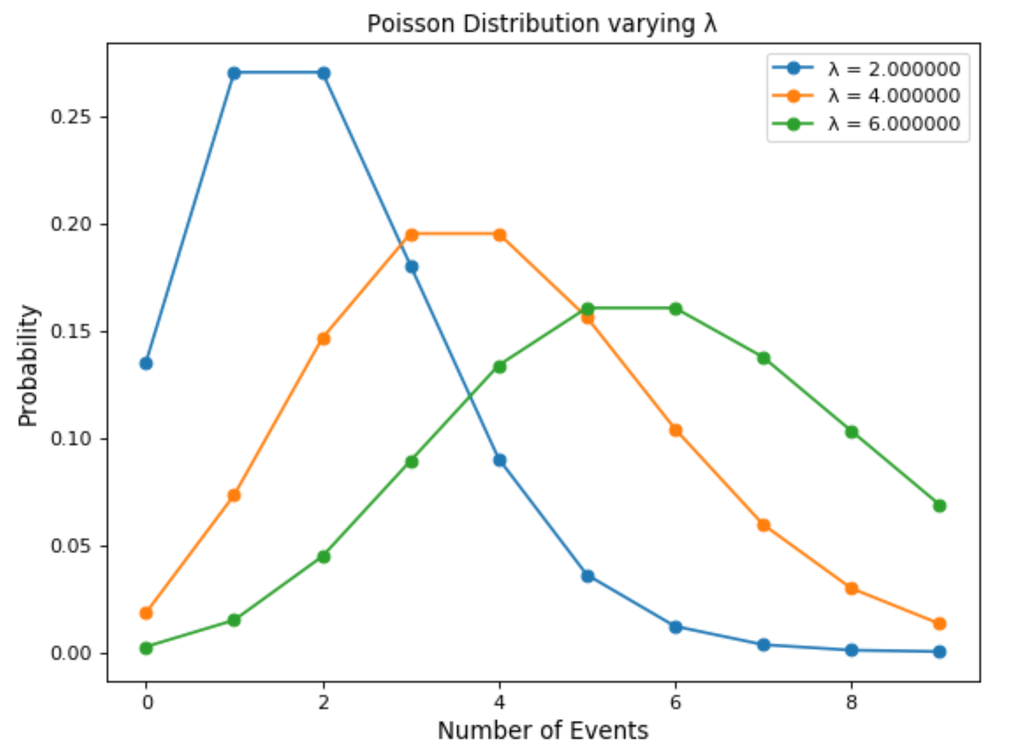
Figure 10: Poisson Distribution varying λ
Exponential Distribution
Finally, the Exponential Distribution is used to model the time taken between the occurrence of different events.
As an example, let’s imagine we work at a restaurant and we want to predict what is going to be the time interval between different customers coming to the restaurant. Using an Exponential Distribution for this type of problem, could be the perfect place where to start.
Another common application of Exponential distributions is survival analysis (eg. expected life of a device/machine).
Exponential distributions are regulated by a parameter λ. The greater the value of λ and the faster the exponential curve is going to decade (Figure 11).
| for lambd in range(1,10, 3): |
| x = np.arange(0, 15, 0.1) |
| y = 0.1*lambd*np.exp(-0.1*lambd*x) |
| plt.plot(x,y, label="λ = {:f}".format(0.1*lambd)) |
| plt.xlabel('Random Variable', fontsize=12) |
| plt.ylabel('Probability', fontsize=12) |
| plt.title("Exponential Distribution varying λ") |
| plt.legend() |
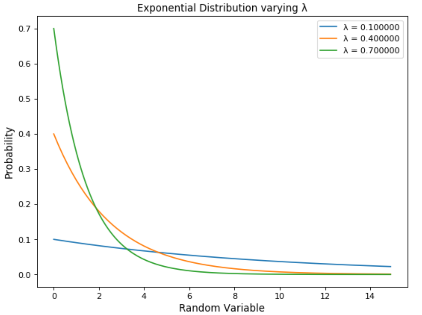
Figure 11: Exponential Distribution
The Exponential Distribution is modelled using the following formula (Figure 12).
Figure 12: Exponential Distribution Formula [6]
If you are interested in investigating how probability distributions are used to demystify Stochastic Processes, you can find more information about it
here.
Contacts
If you want to keep updated with my latest articles and projects
follow me on Medium and subscribe to my
mailing list. These are some of my contacts details:
Bibliography
Bio: Pier Paolo Ippolito is a final year MSc Artificial Intelligence student at The University of Southampton. He is an AI Enthusiast, Data Scientist and RPA Developer.